MonteCarlo模拟

  蒙特卡洛(MonteCarlo)是一种应用随机数来进行计算机模拟的方法。

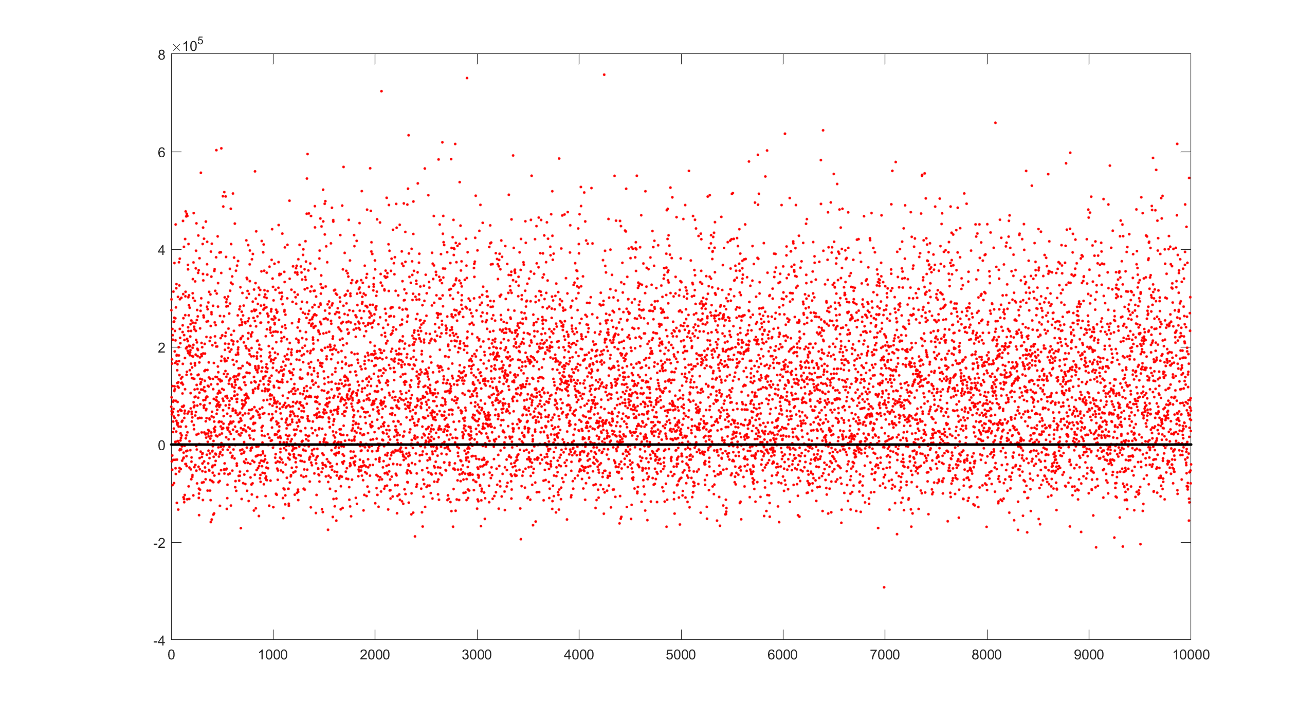
Example1—利润计算

  已知一公司产品售价150元，初期研发成本250000元，单件原材料成本在[50，80]之间波动，市场需求符合正态分布[12000,3000]，单件人工成本成概率出现[(52,0.05)(53,0.25)(54,0.4)(55,0.25)(56,0.05)]。尝试计算公司亏损的概率。

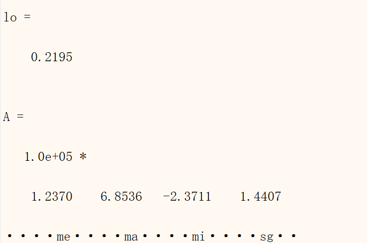
程序

clear
clc
profit=[];
frequency=1000;
for i=1:frequency
    p=150;  %售价
    a=250000;   %广告费
    m=50+(80-50)*rand;  %原材料成本在50-80美元之间均匀分布
    
    r=normrnd(12000,3000);  %符合正态分布
    
    alphabet=[52 53 54 55 56];
    prob=[0.05 0.25 0.4 0.25 0.05];
    l=randsrc(1,1,[alphabet;prob]);     %此函数以‘prob’的概率输出‘alphabet’的值
    
    tp=(p-m-l)*r-a;
    profit=[profit ;tp];    %每运算一次，将上一次的计算结果带入矩阵中
end

me=mean(profit);
ma=max(profit);
mi=min(profit);
sg=std(profit);
po=0;
ne=0;

for i=1:length(profit)
    if profit(i,1)<0        %遍历整个数列，数值小于1则记录1，得到亏损的概率
        ne=ne+1;
    end
end
lo=ne/length(profit)；  %亏损的概率
t=1:frequency;
T=0;
plot(t,profit,'r.',t,T,'black.')

A=[me ma mi sg lo]
disp(['···me··','··ma··','··mi··','··sg··','··lo···'])

结果

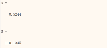
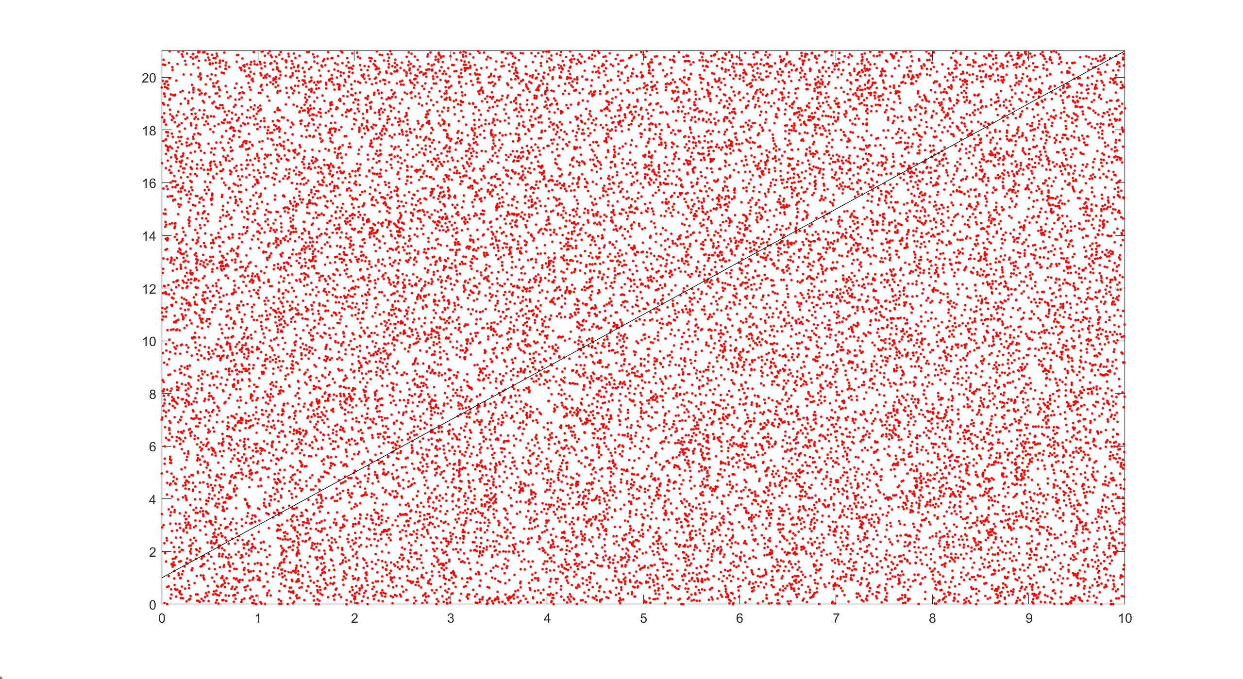
Exercise2—代替积分

  $y=2x+1$,$x \in[0,10]$,求面积。

程序

clear
clc
%用ment carlo算法计算积分
%x[0,10]
%y[0,2x+1]
M=21;
N=10;
j=0;
p=[];
q=[];
frequency=20000;
for i=1:frequency
    m=rand*M;
    n=rand*N;
    if m<(2*n+1)
        j=j+1;
    end
    p=[p;m];
    q=[q;n];
end
s=j/frequency
S=s*M*N

x=[0:10];
y=2*x+1;

plot(q,p,'r.',x,y,'black-')
set(gca,'Ylim',[0,21])

浦松投针问题

  

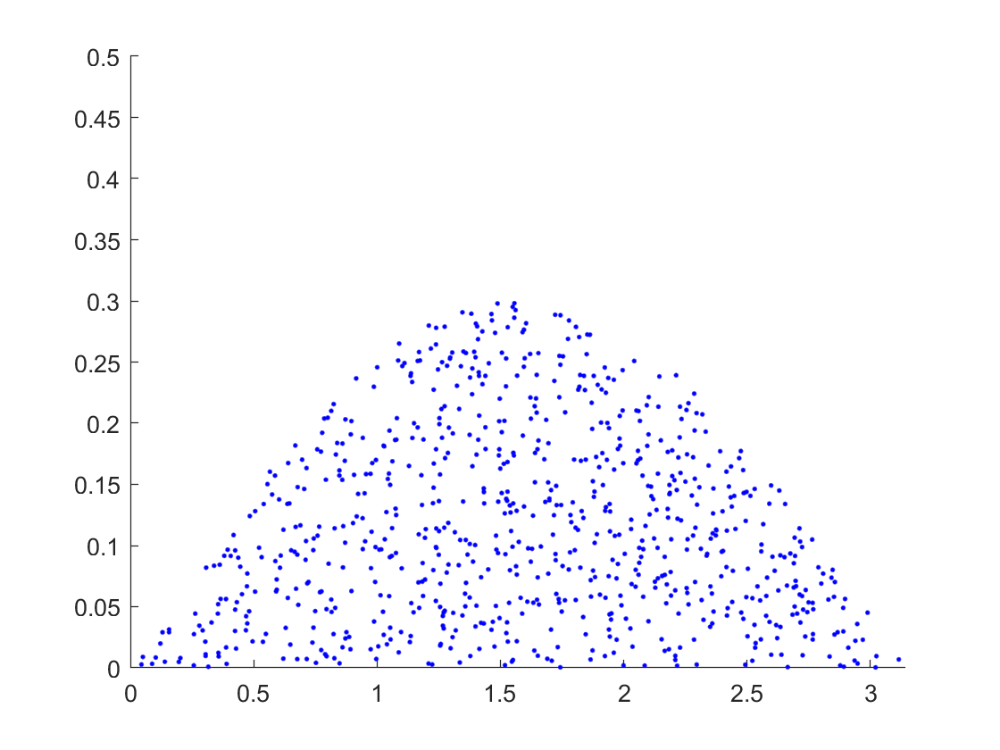
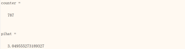
Example—程序

clear
clc
%蒲丰投针实验的计算机模拟
format long;                 %设置15位显示精度
a=1;
l=0.6;                      %两平行线间的宽度和针长
figure; axis([0,pi,0,a/2]); %初始化绘图板
set(gca,'nextplot','add');  %初始化绘图方式为叠加
counter=0;                  %初始化计数器
n=2000;                     %和设定投针次数
x=unifrnd(0,1/2,n,1);       %在[0,1/2]之间产生1*n阶矩阵
phi=unifrnd(0,pi,1,n);      %样本空间Ω
frame=moviein(n);           %建立一个1120列的大矩阵
for i=1:n
if x(i)<l*sin(phi(i))/2  %满足此条件表示针与线的相交
    plot(phi(i),x(i),'b.');
    counter=counter+1;    %统计针与线相交的次数
    frame(:,counter)=getframe; %描点并取帧
end
end

fren=counter/n;
pihat=2*l/(a*fren);%用频率近似计算π
disp(counter);
disp(pihat);

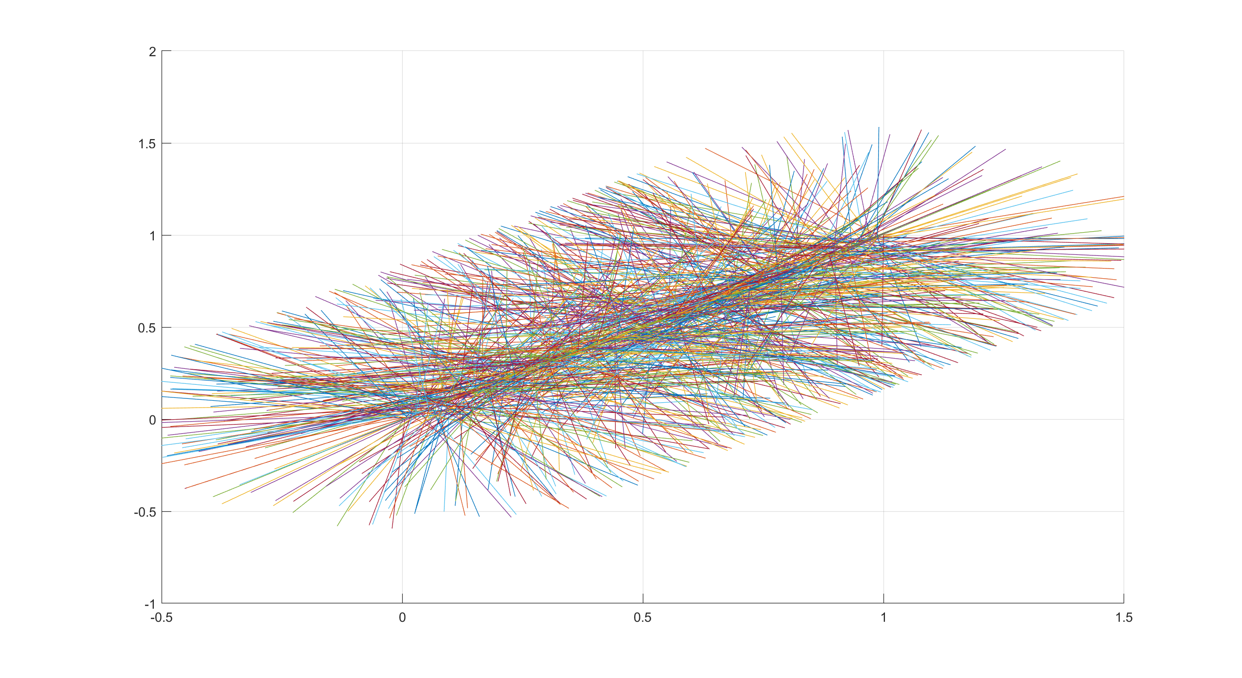
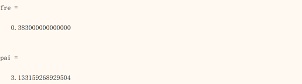
程序

clear
clc
%普松投针--求圆周率
h=1;
l=0.6;
n=10000;
x=unifrnd(0,1,n,1);
y=unifrnd(0,2*pi,n,1);
X=[];
Y=[];
A=[];
B=[];
j=0;
%figure;
%axis([-0.5,1.5,-h,2]); %初始化绘图板
%set(gca,'nextplot','add');  %初始化绘图方式为叠加
for i=1:n
    
    if  x(i)+l*sin(y(i))>=h || x(i)+l*sin(y(i))<0 
        j=j+1;      
    end
    X=[X;x(i)+l*cos(y(i))];
    Y=[Y;x(i)+l*sin(y(i))];
    A=[A;x(i),X(i),Y(i)];
    %plot([A(i,1),A(i,2)],[A(i,1),A(i,3)])
    grid on;
end
A;
fre=j/n
pai=2*l/(h*fre)

输出效果